Basic Neural Network for MNIST with Keras

This is a simple tutorial on a basic 97% accurate neural network model for MNIST digit classification. This model contains multiple RELU layers and dropouts layers with a softmax layer for prediction.

Only less than 30 seconds of training time is required on my 15 inch Macbook. I strongly recommend using jupyter notebook, but normal python terminal is fine too.

# install some libraries if don't have them
pip3 install numpy pandas scipy sklearn tensorflow keras matplotlib

Setting up python environment

import numpy as np
import pandas as pd

import matplotlib.pyplot as plt

Loading data sets

# List our data sets
from subprocess import check_output
print(check_output(["ls", "data"]).decode("utf8"))

# Loading data with Pandas
train = pd.read_csv('data/train.csv')
train_images = train.ix[:,1:].values.astype('float32')
train_labels = train.ix[:,0].values.astype('int32')

test_images = pd.read_csv('data/test.csv').values.astype('float32')

print(train_images.shape, train_labels.shape, test_images.shape)

output:
sample_submission.csv
test.csv
train.csv

(42000, 784) (42000,) (28000, 784)

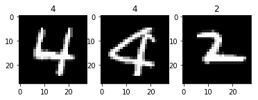
# Show samples from training data
show_images = train_images.reshape(train_images.shape[0], 28, 28)
n = 3
row = 3
begin = 42
for i in range(begin,begin+n):
    plt.subplot(n//row, row, i%row+1)
    plt.imshow(show_images[i], cmap=plt.get_cmap('gray'))
    plt.title(train_labels[i])

Process data for training

# Normalize pixel values from [0, 255] to [0, 1]
train_images = train_images / 255
test_images = test_images / 255

# Convert labels from [0, 9] to one-hot representation.
from keras.utils.np_utils import to_categorical
train_labels = to_categorical(train_labels)

print(train_labels[0])
print(train_images.shape, train_labels.shape)

output:
[ 0.  1.  0.  0.  0.  0.  0.  0.  0.  0.]
(42000, 784) (42000, 10)

Training neural network

# Create a basic neural network
# 64 relu -> 128 relu -> dropout 0.15
# -> 64 relu -> dropout 0.15 -> softmax 10
from keras.models import Sequential
from keras.layers import Dense , Dropout

model=Sequential()
model.add(Dense(64,activation='relu',input_dim=(28 * 28)))
model.add(Dense(128,activation='relu'))
model.add(Dropout(0.15))
model.add(Dense(64, activation='relu'))
model.add(Dropout(0.15))
model.add(Dense(10,activation='softmax'))

from keras.optimizers import RMSprop
model.compile(optimizer=RMSprop(lr=0.001),
    loss='categorical_crossentropy',
    metrics=['accuracy'])

# Train our model with 15 steps using 90% for training and 10% for cross validation
history=model.fit(train_images, train_labels, validation_split = 0.1,
            epochs=15, batch_size=64)

output:
Train on 37800 samples, validate on 4200 samples
Epoch 1/15
37800/37800 [==============================] - 2s - loss: 0.4146 - acc: 0.8743 - val_loss: 0.1901 - val_acc: 0.9419

Epoch 2/15
37800/37800 [==============================] - 2s - loss: 0.1828 - acc: 0.9454 - val_loss: 0.1334 - val_acc: 0.9581

Epoch 3/15
37800/37800 [==============================] - 2s - loss: 0.1359 - acc: 0.9608 - val_loss: 0.1330 - val_acc: 0.9614

Epoch 4/15
37800/37800 [==============================] - 2s - loss: 0.1071 - acc: 0.9680 - val_loss: 0.1217 - val_acc: 0.9671

Epoch 5/15
37800/37800 [==============================] - 2s - loss: 0.0907 - acc: 0.9731 - val_loss: 0.1281 - val_acc: 0.9674

Epoch 6/15
37800/37800 [==============================] - 2s - loss: 0.0774 - acc: 0.9770 - val_loss: 0.1091 - val_acc: 0.9695

Epoch 7/15
37800/37800 [==============================] - 2s - loss: 0.0701 - acc: 0.9799 - val_loss: 0.1146 - val_acc: 0.9712

Epoch 8/15
37800/37800 [==============================] - 3s - loss: 0.0637 - acc: 0.9813 - val_loss: 0.1338 - val_acc: 0.9679

Epoch 9/15
37800/37800 [==============================] - 2s - loss: 0.0594 - acc: 0.9825 - val_loss: 0.1217 - val_acc: 0.9726

Epoch 10/15
37800/37800 [==============================] - 2s - loss: 0.0519 - acc: 0.9851 - val_loss: 0.1245 - val_acc: 0.9736

Epoch 11/15
37800/37800 [==============================] - 2s - loss: 0.0484 - acc: 0.9858 - val_loss: 0.1435 - val_acc: 0.9705

Epoch 12/15
37800/37800 [==============================] - 2s - loss: 0.0451 - acc: 0.9870 - val_loss: 0.1442 - val_acc: 0.9724

Epoch 13/15
37800/37800 [==============================] - 2s - loss: 0.0442 - acc: 0.9872 - val_loss: 0.1412 - val_acc: 0.9702

Epoch 14/15
37800/37800 [==============================] - 2s - loss: 0.0393 - acc: 0.9889 - val_loss: 0.1361 - val_acc: 0.9738

Epoch 15/15
37800/37800 [==============================] - 2s - loss: 0.0398 - acc: 0.9887 - val_loss: 0.1522 - val_acc: 0.9726

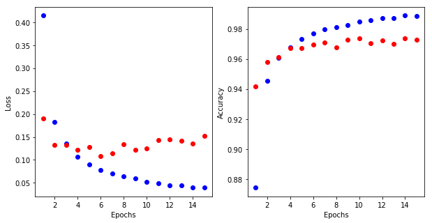
From this output we can see our model is 98.87% accurate on training set and 97.26% accurate on cross validation set.

# Graphing Loss on the left and Accuracy on the right
history_dict = history.history

epochs = range(1, 16)

plt.rcParams["figure.figsize"] = [10,5]
plt.subplot(121)

loss_values = history_dict['loss']
val_loss_values = history_dict['val_loss']
plt.plot(epochs, loss_values, 'bo')
plt.plot(epochs, val_loss_values, 'ro')
plt.xlabel('Epochs')
plt.ylabel('Loss')

plt.subplot(122)

acc_values = history_dict['acc']
val_acc_values = history_dict['val_acc']
plt.plot(epochs, acc_values, 'bo')
plt.plot(epochs, val_acc_values, 'ro')
plt.xlabel('Epochs')
plt.ylabel('Accuracy')

plt.show()

Make prediction

# Generate prediction for test set
predictions = model.predict_classes(test_images, verbose=0)

submissions=pd.DataFrame({"ImageId": list(range(1,len(predictions)+1)),
                         "Label": predictions})
submissions.to_csv("predictions.csv", index=False, header=True)

Everything all together takes about 5 minutes, pretty good for 97% accuracy. There are many ways to improve the accuracy, I might write about them in future. The goal here is just to have a basic working setup and test submissions on Kaggle.

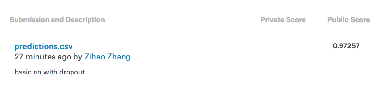
With this simple model we achieved 97.257% accuracy on test set.

Thanks Poonam Ligade for posting her Kaggle Kernel

Try this problem on Kaggle